Nothing So Practical

Causal Inference Is Hard

The first post argued that causal inference is simply a matter of ruling out rival explanations. That sounds pretty straightforward, but it’s not. Rival explanations can be hard to identify, hard to measure, and hard to eliminate. Overlook a confound, measure it poorly, or choose an inadequate study design, and causal inference fails. No matter how sophisticated the method, the model will estimate the treatment effect you ask for. When causal inference fails, it fails silently.

Rock Me Amadeus

In 1993, researchers reported that listening to Mozart for 10 minutes improved spatial reasoning, compared to a relaxation tape or silence. Headlines announced that Mozart makes you smarter. Baby Mozart CDs appeared and some states even passed legislation encouraging classical music for children.

The conditions in the original study didn’t just differ in the presence of Mozart. They also differed in arousal and mood. Subsequent studies found that other enjoyable stimuli (e.g., Schubert, a Stephen King story) produced similar boosts, and that the effect disappeared when researchers controlled for positive affect. The active ingredient seemed to be a stimulating experience, not Mozart.

The confound wasn’t statistical, it was conceptual. Comparing Mozart to silence doesn’t isolate the effect of Mozart. It confounds music with the psychological experience of music: engagement, pleasure, stimulation. The researchers wanted to test the effect of music on spatial reasoning, but the comparison tested whether an engaging experience outperformed a boring one.

It took several follow-up studies to catch this. The confound was invisible to the p-values. It could only be seen by thinking carefully about what the comparison actually tested.

99 Rivals

The Mozart study was a controlled experiment, and a confound still slipped through. In observational studies with little control, the threats only multiply. Identifying them requires knowing the subject matter well enough to see what else could be driving the result.

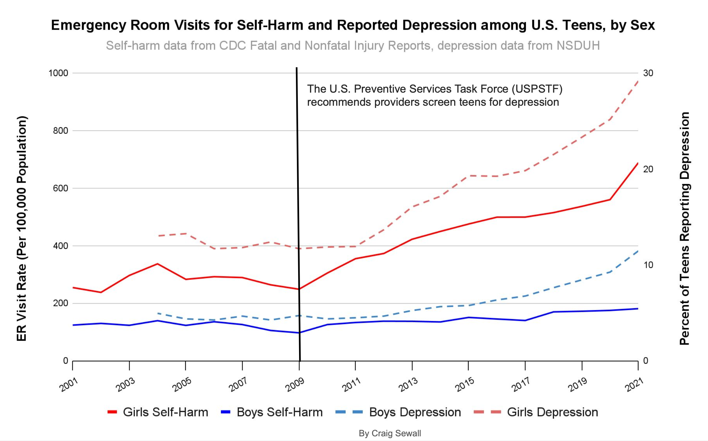
The relationship between smartphones and teen mental health is a case in point. Starting around 2012, surveys showed rates of anxiety, depression, and self-harm increasing among adolescents. Smartphone adoption was also accelerating in that period. The timing lines up, and the causal story practically writes itself. But “seems obvious” is where observational research goes to die. There were numerous events around that time that could generate similar patterns.

The Great Recession’s aftermath left families under sustained economic stress into the 2010s. Academic pressure intensified as college admissions grew more competitive. School shootings became a recurring feature of adolescent life. These are history effects, events external to the treatment that coincide with it and could independently produce the observed outcome. They aren’t visible in the dataset.

Then there are the changes in how the outcome itself is measured. In 2009, routine depression screening was recommended for adolescents, and the following year the Affordable Care Act required insurers to cover it. More screening produces more diagnoses, even if the underlying rate hasn’t changed. Coding changes in how hospitals recorded suicidal ideation had a similar effect. Add destigmatization that makes teens more willing to report mental health struggles, and you have an outcome variable that can shift for reasons entirely unrelated to smartphone use.

This is not to say that smartphones are harmless.¹ The point is, observational evidence can’t cleanly separate the smartphone signal from the noise of everything else that changed. And even if you could identify every last one, you’d still need to measure them well enough to neutralize confounding. That turns out to be its own problem.

Measuring the Weight of Smoke

In the HRT example from the first post, we identified health consciousness as the key confound. Measuring it is harder than it sounds. The Nurses’ Health Study collected data on diet, exercise, smoking, alcohol use, preventive care visits, and vitamin consumption. The groups still weren’t comparable. Health consciousness isn’t a checklist of behaviors. It’s a disposition that leads someone to ask their doctor about hormone therapy. The studies captured visible markers but missed the trait that drove both HRT use and cardiovascular health. Controlling for the markers didn’t eliminate the alternative explanation.

Many confounders that matter are abstract constructs. Motivation, risk tolerance, management quality, organizational culture. Even if you identify them all, you still have to measure them well. If health consciousness has three dimensions and you only capture two, the unmeasured dimension still pollutes your result. This is where many studies quietly unravel. The model runs without complaint, and the confounding goes undetected.

By Dint of Design

Instead of trying to measure every confounder, you can use a study design that neutralizes them structurally. Difference-in-differences (DiD) illustrates this logic. Rather than comparing HRT users to non-users at a single point in time, we compare how each group’s outcomes changed. If health-conscious women consistently have better cardiovascular outcomes, that gap is the same in both periods and gets differenced out. This eliminates any stable baseline difference between groups, including unmeasured ones.

Design-based approaches trade one assumption for another. For DiD, we trade “no unmeasured confounding” for the assumption that treated and untreated groups would have followed the same trend without the treatment. That’s less demanding, but the parallel trends assumption can’t be verified where it matters most: the post-treatment period you never get to observe. You can check for parallel trends before treatment, but that doesn’t guarantee parallel trends after.

Suppose that around the same time HRT became a popular treatment, public health agencies launched cardiovascular screening campaigns targeting women. Women on HRT might show decreasing heart disease trends not because of hormone therapy, but because they were getting screened and treated earlier. The design would attribute the improvement to HRT when it belonged to the screening campaign.

Using design shifts the burden from measurement to plausibility, but it doesn’t eliminate the burden. And all of this assumes you’ve correctly identified what the treatment actually is.

Free Bird

Even sophisticated methods can trip over an ambiguous treatment. Hours after Elon Musk closed his acquisition of Twitter, he tweeted “the bird is freed.” Molak used this event to demonstrate synthetic control, a method that constructs a counterfactual by weighting comparison time series to match the pre-treatment trajectory of the treated unit. Any post-treatment divergence is attributed to the treatment. The model estimated a large effect of Musk’s tweet on Google searches for “Twitter.”

This was a sound application of a contemporary method. The effect was large with a clear divergence at the treatment. But as the author correctly notes, “the outcome might be influenced not only by Musk’s tweet but also by other factors (e.g. media publications on Twitter acquisition).” The acquisition dominated the news cycle for days before. People were already searching for “Twitter” because of news about the takeover. Information about Musk’s acquisition of Twitter and his tweet weren’t independent.

A degraded fit in the period before the tweet might suggest that the baseline was contaminated by acquisition news. But the treatment definition problem is invisible to any diagnostic. The model is answering the question, “what would searches look like without this event?” but “this event” isn’t one tweet. It’s major news that generated weeks of coverage. The model can’t distinguish the tweet from the acquisition because they’re the same story.

The model answered the question it was given; the data just weren’t suited to that question. The only way to catch it is by considering what else was happening when the “treatment” occurred. That’s domain knowledge, not statistics.

The Real Work of Causal Inference

Each example above follows a similar pattern. A credible method produced a reasonable result that looked clean but wasn’t. These aren’t cautionary tales about unskilled researchers. They illustrate how causal inference actually works. The methods do what you ask. But every method operates under assumptions, and assumptions are claims about the world, not properties of the estimator. When they don’t hold, the estimate is confounded regardless of what the output says.

The hard work of causal inference isn’t technical, it’s substantive. It requires thinking carefully about mechanisms and processes, not just running regressions and checking p-values. Studying cognitive performance requires understanding the influence of arousal and mood. Understanding the impact of smartphones on teen mental health requires knowing about changes in screening policy, insurance coverage, and diagnostic coding. Estimating the impact of a tweet on search behavior requires awareness of media coverage and news cycles.

Technical frameworks are valuable precisely because they make reasoning about causal questions explicit and systematic. Researchers are forced to articulate their assumptions about the data generating process. They provide formal rules for translating those assumptions into valid causal estimates. They provide a check on whether your logic is internally consistent. But they really only work if you understand the domain you’re studying. No amount of technical sophistication can substitute for that knowledge.

Causal inference ultimately comes down to knowing the subject matter well enough to identify the ways you could be wrong, then using study design or statistical methods to rule them out. DAGs and potential outcomes help ensure rigor in the latter. But identifying how you could be wrong requires expertise that no equation or code can provide. Causal inference is easy once you understand this. Actually doing it well? That’s the hard part.

References

Corredor-Waldron, A., & Currie, J. (2024). To what extent are trends in teen mental health driven by changes in reporting? The example of suicide-related hospital visits. Journal of Human Resources, 59(S), S14–S40.

Nantais, K. M., & Schellenberg, E. G. (1999). The Mozart effect: An artifact of preference. Psychological Science, 10(4), 370–373.

Rauscher, F. H., Shaw, G. L., & Ky, K. N. (1993). Music and spatial task performance. Nature, 365, 611.

Pew Research Center. (2015). Teens, social media & technology overview 2015. https://www.pewresearch.org/internet/2015/04/09/teens-social-media-technology-2015/

Thompson, W. F., Schellenberg, E. G., & Husain, G. (2001). Arousal, mood, and the Mozart effect. Psychological Science, 12(3), 248–251.

Twenge, J. M. (2020). Increases in depression, self-harm, and suicide among U.S. adolescents after 2012 and links to technology use: Possible mechanisms. Psychiatric Research and Clinical Practice, 2(1), 19–25.